Énoncé
ABCDEFGH est un cube d'arête 1.
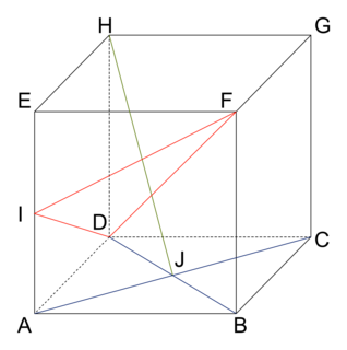 |
On a placé les points I, J tels que :
• I milieu de [AE] ;
• J centre de la face ABCD.
PARTIE A
Le but de cette partie est d'étudier la position relative de la droite (BH) et du plan (IDF) en utilisant le produit scalaire, sans et avec un repère.
1.
On rappelle que la longueur de la diagonale d'un carré de côté 1 est égale à  .
.
.a. En remarquant que  et que
  calculer
  .
.
et que calculer .b. En utilisant la même méthode, calculer  .
.
.c. En déduire les positions relatives de la droite (HJ) et du plan (IDF).
2.
On se place dans le repère orthonormé  .
.
.a. Donner les coordonnées de tous les points de la figure.
b. Donner les coordonnées des vecteurs  et
et  En déduire
  .
.
et En déduire .c. En utilisant la même méthode, calculer  .
.
.d. En déduire les positions relatives de la droite (HJ) et du plan (IDF).
PARTIE B
Le but de cette partie est de donner une mesure de l'angle  .
.
On se place de nouveau dans le repère orthonormé .
.
.On se place de nouveau dans le repère orthonormé
.1. Calculer les longueurs ID, IF et DF.
2. Calculer le produit scalaire  de deux manières différentes pour en déduire l'angle
  arrondi au degré près.
de deux manières différentes pour en déduire l'angle arrondi au degré près.La bonne méthode
PARTIE A
1.
a. Utiliser deux propriétés du produit scalaire, la distributivité et l'orthogonalité de deux vecteurs.
b. Utiliser la relation de Chasles en introduisant les points D et A.
c. Déduire des questions précédentes l'orthogonalité de vecteurs.
2.
a. Lire les coordonnées sur la figure.
b. Utiliser la définition des coordonnées d'un vecteur dans un repère orthonormé et la définition du produit scalaire dans un repère : soient  et
et  deux vecteurs de l'espace, alors
et deux vecteurs de l'espace, alors c. Même méthode qu'au b.
d. Même conclusion qu'au 1.c.
PARTIE B
1. Utiliser la formule de calcul de distance dans un repère orthonormé de l'espace.
2. Utiliser la définition générale du produit scalaire  et la définition dans un repère.
et la définition dans un repère.Corrigé
Partie A
1.
a. 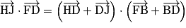

Or car les deux vecteurs sont égaux,
  et
et  car les vecteurs sont orthogonaux.
De plus,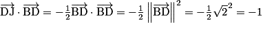 , car J milieu de [BD].
Donc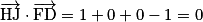 .
.
Or
car les deux vecteurs sont égaux, et car les vecteurs sont orthogonaux.De plus,
, car J milieu de [BD].Donc
.b. 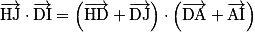

Or et
et  car les vecteurs sont orthogonaux,
 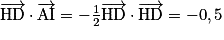 car I milieu de [AE].
De plus, on a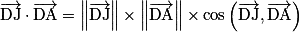 .
.
 .
.
Donc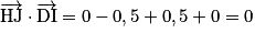 .
.
Or
et car les vecteurs sont orthogonaux, car I milieu de [AE].De plus, on a
..Donc
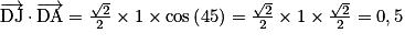
.c. Le plan (IDF) admet  et
et  comme vecteurs directeurs. Or
  et
et  , donc
  est un vecteur normal au plan (IDF).
Par conséquent, la droite (HJ) est orthogonale au plan (IDF).
et comme vecteurs directeurs. Or et , donc est un vecteur normal au plan (IDF).Par conséquent, la droite (HJ) est orthogonale au plan (IDF).
2.
a. On a 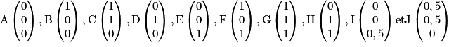 .
.
.b. On a 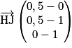 donc
donc  .
.
De même, on a donc
donc  .
.
Ainsi, on a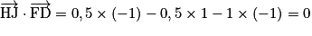 .
.
donc .De même, on a
donc .Ainsi, on a
.c. On a 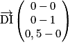 donc
donc  .
.
Ainsi, on a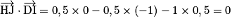 .
.
donc .Ainsi, on a
.d. Le plan (IDF) admet  et
et  comme vecteurs directeurs. Or
  et
et  donc
donc  est un vecteur normal au plan (IDF).
Par conséquent, la droite (HJ) est orthogonale au plan (IDF).
et comme vecteurs directeurs. Or et donc est un vecteur normal au plan (IDF).Par conséquent, la droite (HJ) est orthogonale au plan (IDF).
Partie B
1. 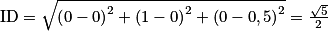 .
.
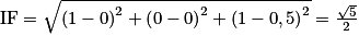 .
.
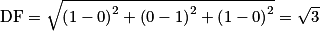 .
.
...2. On a  et
et  Donc
Donc 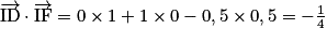 .
.
De plus,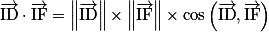 .
.
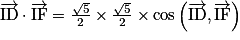 .
.
Donc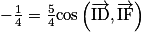 d'où
d'où  .
.
On a donc .
.
et Donc .De plus,
..Donc
d'où .On a donc
.